Power Laws in the Stock Market

Reference journals:
https://pubs.aeaweb.org/doi/pdf/10.1257/jep.30.1.185
https://www.sas.upenn.edu/~fdiebold/papers/paper39/ABDE.pdf

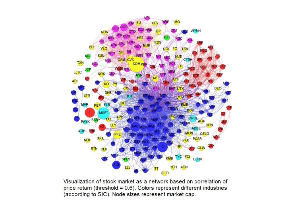
For purposes of maximizing profits and minimizing risk in stock markets, many traders seek to model the stock market as accurately as possible. Recently (<100 yrs), index investment has grown in popularity over investments in individual stocks (index investment is a strategy of investing in a broad market or range of stocks). The reason can be explained using power laws.

In almost every major market benchmark such as the S&P500, the top 20% of stocks, in terms of market cap and trade volume, represent approximately 85% of the total market size. More interestingly the same pattern appears in the distribution of market returns. The top 20% of stocks represent approximately 80% of the market’s year-on-year return (on average). This inequality is graphically similar to the long-tailed graphs we saw in class; in other words, the distribution of returns in the stock market is a long-tailed power law distribution. And according to the author’s research, it is in fact consistent with

P(x > X) ~ 1/X^a , with a = 3 : an inverse cubic power law

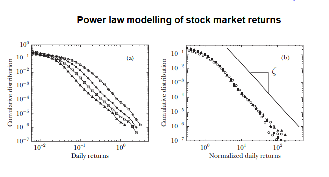
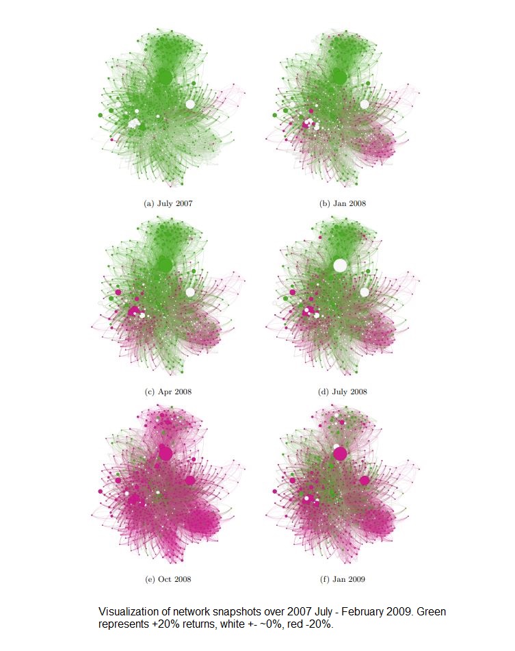
This formula is consistent with the one we discussed in class: p(x) = x^-a. It is also consistent with our discussion of the value of alpha (the a value) which we discussed to mostly be 2 < a < 3 . This is interesting but why is it important? This is important because since stock markets follow power law distributions instead of something like a Gaussian, extreme variations in day-to-day prices (such as crashes) are very rare. Because of the cubic law behavior of markets the chances of a stock price deviating from the mean by 10% is 1000 times less than if market returns were instead Gaussian. And we can see this in practice, on average only 1 out of 1000 stocks on any given day on the NYSE deviate by 10% (which means the market is relatively stable, which is good).

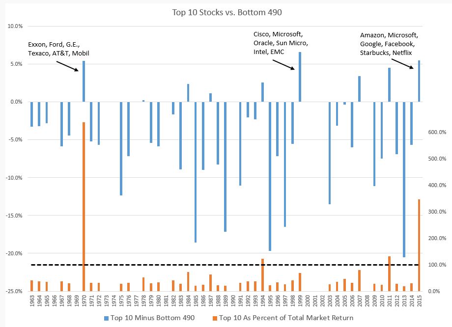
This modelling of power laws is also leads to strategies for trading. Traders can either aim to pick or not pick the stocks that tend to deviate more. In a good economy, perhaps they will pick the few stocks that are on the extreme tail of the power law distribution, and oppositely in a bad economy. Example being in 2015 when the S&P500 would have ended the year with negative growth if it were not for 10 stocks and F.A.N.G (FANG = Facebook, Apple, Netflix, Google). Conversely, during the tech bubble burst, you would not have wanted to pick these stocks. In class we briefly discussed models that lead to power laws. It turns out that the random walk model is what makes stock returns a power law distribution.

Any blue bar above the 0.0% line means that for that year, the top 10 stocks in terms of growth out-contributed the rest of the 490 stocks combined (S&P500). Note in years like 2015 and 2000, without the top 10 stocks, the market would have experienced negative growth. This extremity in contribution represents in bar graph form the power law distribution of stock market returns.

Going back to why index investment is gaining popularity — because according to the distribution of market returns, it is safer to diversify instead of pinpoint specific stocks. Investing in stocks from the tail (extreme deviations) only works when times are good, and because it is very difficult to predict good/bad times, money managers often make the safe play of diversifying (game theory!).

Overall it is interesting to see how the theory of power laws we covered in class are represented in society because sometimes it is not immediately obvious as to why power laws would model certain things — such as the stock market since for the most part the market grows and shrinks randomly.

Reference List

Gabaix, Xavier. “Power laws in economics: An introduction.” Journal of Economic Perspectives 30.1 (2016): 185-206.

Andersen, Torben G., et al. “The distribution of realized stock return volatility.” Journal of financial economics 61.1 (2001): 43-76.

Network Analysis of the Stock Market

In class we have discussed many properties of graphs including clustering, graph connectivity, and degree centrality and connectedness. In this blog I will outline the real world use of these properties in stock market analysis.

There have been many attempts to “beat” the stock market for obvious reasons ($). Traditional approaches such as technical and fundamental analysis have their believers and critics. Another approach, based on graph theoretical analysis, is also used in risk analysis and portfolio management. By nature the stock market is correlated because we live in a global economy — no company is isolated. Thus stock markets can be represented as a cluster of companies with edges forming between companies sharing a characteristic. Here we focus on the representation of the stock market as a network based on correlated stock returns. That is, If the absolute difference between the return of two stocks is less than some defined threshold theta, an edge is formed between them.

An interesting result is that after applying community detection algorithms on such a network (such as the Girvan-Newman algorithm as discussed in class), the resulting clusters were consistent with the market classifications as denoted by the Standard Industrial Classification (SIC) system; a classification of industries by 4-digit code. This illustrates that stocks within similar sectors tended to perform similarly. In class we refered to this as communities sharing the same behaviors or “birds of a feather are alike”. Using software to visualize stock return correlations offers an intuitive way to analyze the overall structure of a set of stocks, and to helps to identify key companies/market clusters — this is an important aspect of risk analysis/portfolio management.

This networking model can be applied to stocks listed on the S&P 500 based on rate of return over the time frame July 2007 – February 2009. Snapshots of the network can be taken at smaller time frames i.e July 2007 – August 2007, August 2007 – September 2007, etc. to produce a series of networks depicting the progression of correlation between companies. The interesting result is that looking at the series of networks, you can observe a ‘cascading’ or spreading effect of returns in clusters. This is similar to what we discussed about network security and the spread of malicious software. Thus this network representation of the stock market could be useful in systemic risk and cascade effects prediction.

Note: this time frame represents the approximate timeline of the US Financial Crisis in ’08

Notice the ‘cascading’ effect along the graph at each time frame and how it spreads along clusters

Why network analysis over traditional methods?

Traditional approaches tend to rely on statistical properties such as variance and expected returns over time. However these typically represent localized behavior of one or two stocks and do not represent the behavior of a cluster/community of stocks. A network representation that characterizes stocks in clusters of connected components (industries) gives insight to more macro properties of the market. Properties such as degree centrality and betweeness of a stock can be identified.

A practical example is if Apple (AAPL) suddenly loses 50% of its value: semiconductor, glass screen, and other electronic hardware companies will almost surely experience similar losses soon after in a cascading effect. Network analysis can help to identify these clusters.

Limitations

Note this doesn’t mean you can beat the market with network analysis. Limitations of network analysis are that it doesn’t actually quantify how to actually achieve a better portfolio. Yes it can tell you to diversify so that your portfolio isn’t comprised of stocks all from one cluster, but ultimately it does not consider how much of each stock, at what time frame, and at what prices would be optimal points of entry/exit. Perhaps network analysis properties such as stock connectedness could be used in conjunction with a neural network to formulate a quantitative approach to optimize some return function of dollars.

References

[1] Huang, Wei-Qiang, Xin-Tian Zhuang, and Shuang Yao. “A network analysis of the Chinese stock market.” Physica A: Statistical Mechanics and its Applications 388.14 (2009): 2956-2964.

[2] Sun et al., 2015. Sun, W., Tian, C., and Yang, G. (2015). Network analysis of the stock market.

[3] 许忠好, and 李天奇. “基于复杂网络的中国股票市场统计特征分析.” 山东大学学报 (理学版) 52.5 (2017): 41-48.

Photos courtesy of [2].