Author: Jason Zhong

In epidemics there is the basic reproductive number R_0 is crucuial in determining if epidemics can blow up or die out. Ideally we want R_0 to be below 1 in order for the epidemic to die out. One way would be to reduce p, the probability of infection. Vaccines seem like an obvious and simple way to reduce p, however not everyone gets vaccinated. A recent study published this year called, Epidemic prevalence information on social networks can mediate emergent collective outcomes in voluntary vaccine schemes, analyzes the effect of vaccination on epidemics while using game theory.

Getting vaccinated can be viewed as a payoff matrix. Getting vaccinated requires time which many value more. On the other hand, herd immunity can still protect unvaccinated individuals at no cost as long as enough of the population is sufficiently vaccinated.As a result, many individuals may choose to not get vaccinated but still be protected by vaccines because there are less infectious people. For rational agents, it may seem disadvantagous to sacrifice time to get vaccinated when the individual still benefits from herd immunity regardless.

In the study researchers studied the dynamics of epidemic spreading and vaccine uptake behaviour on a social network containing N people. The model uses the popular SIR epidemic model with transmission rate β, and average infectious time period of τI. In the study they varied the transmission rate and average time period. One unique aspect of the model is the introduction of vaccinations, which prevents susceptible individuals from being infected, which makes them functionally similar to recovered individuals.

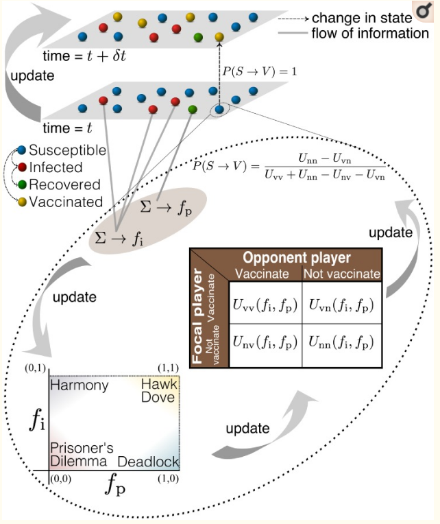
Individuals have access to local information such as number of infected cases among direct contact neighbours in the network, and global information about how prevalent the disease is across the whole network. The player’s payoff matrix evolves as time passes, since the payoffs are based on the disease prevalence, where a higher prevalence of diesease increases the payoff for getting vaccinated. Interestingly, the payoff to not vaccinate increases as the number of direct neighbours are vaccinated or immune to the disease.

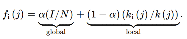
The formula for the payoff of vaccination scales based on α∈ [0, 1], which is a weight factor determining the impact of global vs local information. For example, if α=1, then individuals only considers global information on the epidemic when determing the payoff matrix for vaccinate/don’t vaccinate, but if α=0 then the individuals only consider local information.

The results of the 1000 epidemic simulations with β= 0.025 , τ_I = 10, and α=0 or α=1 are shown above. When α=1 people don’t initially get vaccinated, but when the epidemic becomes significantly higher then there is a mass surgence of vaccinations, akin to how media exposure only occurs when epidemics grows large which in turn can trigger vaccinations. Also, the fraction of infected, inf_∞, is always higher in α=1 regardless of R_0, which is in line with the observation that people get vaccinated based on global epidemic data. This may suggest that dispersing local information about epidemics is more important than global information.

This study shows the importance of information dispersal in combatting epidemics. The results may suggest more efficient disease control by providing local information. It is also interesting to note how payoff matrices can change in relation to the environment.

Links:

https://www.ncbi.nlm.nih.gov/pmc/articles/PMC6532839/

As we have learned in class we can represent data in the form of networks which we can use to better understand systems. One such useful application of networks is in the analysis of how disease spreads among the population. One study from 2005 called “The Impacts of Network Topology on Disease Spread” uses various random networks to do just that.

In the study it randomly generated four different types of networks of 500 nodes with similar amount of edges, but randomly assigned. The following types of networks were exactly like the ones we learned in class:

(i) – The Erdős–Rényi model (1960) which we learned in class as G_np. As we know these random networks have low clustering coefficients and a binomial degree distribution.

(ii) – Regular lattices where each node is connect to k nearest neighbours to form either a grid of an array. These networks has a high clustering coefficient, but relatively high average path length since nodes only connect to their nearest neighbours.

(iii) – Rewired lattices (Watts-Strogatz 1998) where we start with a low-dimensional lattice (grid or array) and rewire to introduce randomness (“shortcuts”). By rewiring this introduces more clustering and short paths, thus lowering the average path length.

(iv) – Scale-free networks that have a power-law tail in their degree distribution. These networks have small average path lengths and low clustering.

The following are the properties of the various networks randomly generated with a set amount of vertices (nodes) and similar amount of edges. It is interesting to note that the average path length.

Network type	n (vertices)	M (edges)	K (degree)	C (clustering)	D (length)	S (significance)
Random graph (RG)	500	1905 (33.9)	7.62 (2.71)	0.02 (0.00)	5.67 (2.19)	4.47 (0.25)
Scale-free network (SF)	500	1990	7.96 (8.18)	0.07 (0.00)	2.93 (0.02)	5.60 (0.04)
1D lattice (1D)	500	2000	8.00	0.64	31.69	1.39
2D lattice (2D)	500	1865	7.46	0.23	8.00	1.84
Rewired 1D lattice (1DR)	500	2000	8.00 (0.35)	0.62 (0.00)	8.19 (0.45)	1.59 (0.02)
Rewired 2D lattice (2DR)	500	1865	7.46 (0.33)	0.21 (0.00)	4.95 (0.05)	1.96 (0.01)

The nodes in these networks representing susceptible individuals to diseases and the edges representing a potential method of transmission for the disease. An infected node has a certain probability to infect all its neignbours after each time step. After a node infects another node, there is a time delay until that node becomes capable of infecting other nodes. Even after that, there is a time latency until an infected node becomes immune to the disease, thus non-infectious. Initially one node is infected in a network and the researchers analyzed how the disease spread through the network. They ran many simulations with varying infection probability on all of the types of graphs found that network types had an impact on how fast the epidemic spread. From fastest to slowest rate of infection:

1. Scale-free network
2. The Erdős–Rényi model (1960) (G_np )
3. Rewired 2D lattice
4. 2D lattice
5. Rewired 1D lattice
6. 1D lattice

It is interesting to note that scale-free networks resulted in the largest epidemics for any level of infection. It reached the maximum epidemic size of 500 sooner than the other networks for any probability of infection. 1D lattices never reached the max epidemic size and grew linearly.

It is important to ask why is it that epidemics spread quickly in scale-free networks but spread poorly in 1D lattice networks. The high average path length in 1D lattices and low average path length in scale-free networks helps explain that. In 1D lattices the high average path lengths prevents the infectious nodes from spreading the infection to distant clusters. The infection only grows outwards from the inital cluster. In scale-free networks, the low average path lengths enable infectious nodes to infect far away clusters which help quicken the spread of the infection. It now becomes clear why the rewired 2D lattice and rewired 1D lattice spread infections better than their non-rewired counterpart. The rewiring introduces more shortcut paths which lower the average path length which helps spread the infection faster.

Although the these were simulations on randomly generated networks, they show how understanding networks, random networks in this case, can help us understand real life problems.

References:

Shirley, Mark D.f., and Steve P. Rushton. “The Impacts of Network Topology on Disease Spread.” Ecological Complexity, vol. 2, no. 3, 2005, pp. 287–299., doi:10.1016/j.ecocom.2005.04.005.