During the 1960’s in America, every US based tobacco company was heavily advertising on TV. Warnings were issued by the government about tobacco use and it’s hazardous effects. The US government did not want cigarettes being advertised on TV due to these effects, and subsequently banned cigarette advertising on TV in 1971. We will examine how the Prisoner’s Dilemma that we learned about in class can be applied here. This relates to the class material as it is a real life application of the Prisoner’s Dilemma.
Say we have two cigarette companies; Reynolds, and Philip Morris. Each company has two choices; to advertise or not to advertise. The payoff in this case is the profit that each company can make. For example, if both do not advertise, then each company earns $50M profit. To advertise costs $20M, and with this, the company that advertises gains $30M in sales from their competitor’s profits. If both companies advertise, they both get the same amount of sales, and the profit for each company is $30M ($50M-$20M). The following table represents the payoff matrix.
If we were to look at Reynold’s perspective; if Philip Morris advertises, then we should advertise too, since we would make $30M, compared to $20M if we were to not advertise. If Philip Morris does not advertise, then we should advertise again in this case, since we would make $60M, compared to $20M. This is similar to the Prisoner’s Dilemma that we looked at in class. In this case, advertising is the dominant strategy as it gives the most profit no matter what the other company does.
Prior to the 1971 ban, both companies were heavily advertising, displaying the bottom right outcome. After the 1971 ban on cigarette advertising took place, the only possible scenario that was left was the top left outcome. As a result of this, advertising costs were significantly down, and profits were significantly up, as expected from the payoff matrix. In this case, the government’s hand helped to increase profits for both companies.
References:
Qi, Shi. “The Impact of Advertising Regulation on Industry: The Cigarette Advertising Ban of 1971.” The RAND Journal of Economics, vol. 44, no. 2, June 2013, pp. 215–48. https://doi.org/10.1111/1756-2171.12018
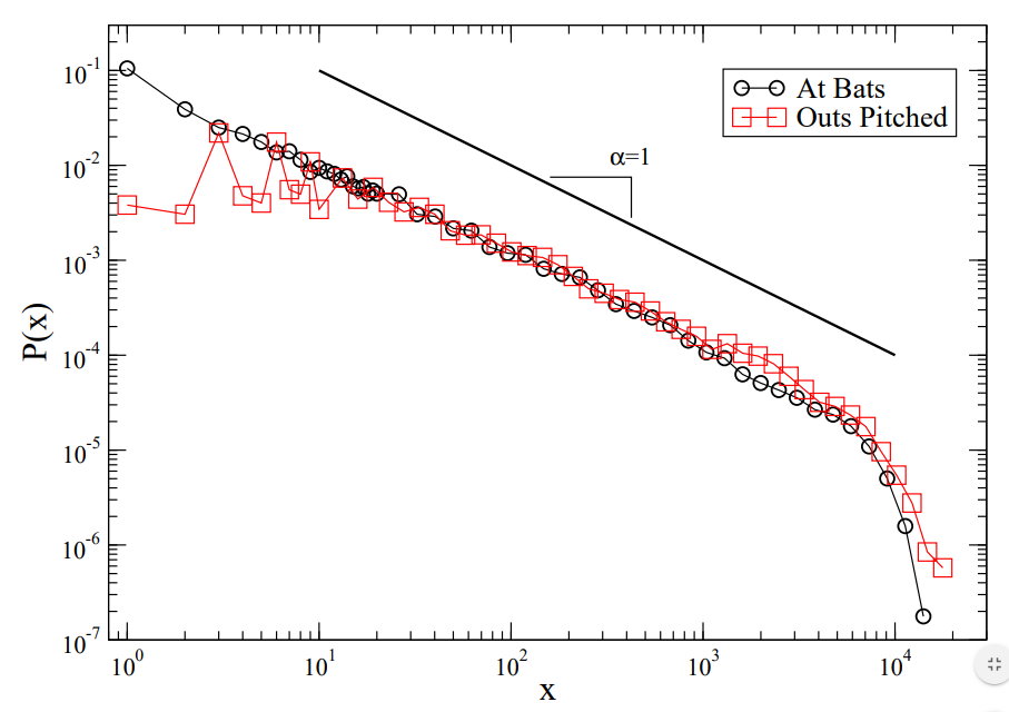
We have seen power law applications arise naturally in many applications with networks, and it also appears in a sport heavily studied by statisticians: baseball. Researchers at Boston University found that the length of player careers in Major League Baseball (both pitchers and batters) followed a power law distribution (Petersen, Woo-Sung, & Eugene, 2008). The study recorded all players with careers ending between the years 1920 and 2000.
Baseball like many other professional sports, is incredibly competitive. What makes baseball unique to other team sports is that there is a team dynamic, but there are many individual battles between pitchers and batter which can determine the outcome of a game. In the study measured to determine typical major league career longevity, both pitchers and batters were found to have similar projected career longevity. I found this surprising, considering how we hear of pitchers facing serious, sometimes career-ending arm injuries. Career longevity was measured using a similar metric for both pitchers and batters, with pitcher longevity measured in number of innings pitched, and batter longevity in number of at-bats.
In terms of power law distribution, the “heavy-tail” part of the distribution was for players with extremely short careers of only a few games, for both pitchers and batters. By contrast, there were very few players who maintain long careers. The longevity of all these players careers were affected by similar factors.
Probability density function of player career lengths
The greatest factors were suspected to be the league’s relatively long regular season compared to other sports (162 games), and the competitiveness of the league. Due to the long regular seasons, players often play games with limited rest, and require occasional substitution with less skilled players for some games. In addition, temporary injuries to regular players during the season allow for new players to break out of the minors and enter the league as a temporary replacement. However, many of these new players do not maintain long careers as they are not sufficiently skilled to remain in the league, accounting for many players having very short (a handful of games) careers.
The greatest factors were suspected to be the league’s relatively long regular season compared to other sports (162 games), and the competitiveness of the league. Due to the long regular seasons, players often play games with limited rest, and require occasional substitution with less skilled players for some games. In addition, temporary injuries to regular players during the season allow for new players to break out of the minors and enter the league as a temporary replacement. However, many of these new players do not maintain long careers as they are not sufficiently skilled to remain in the league, accounting for many players having very short (a handful of games) careers.
The same injuries to players also affect player longevity, where some injuries can be career-ending, others cause small reductions in performance. Since the league’s competitiveness level remains consistent, as players age, and/or develop more injuries, they may no longer be competitive enough to remain in the league. Highly skilled players who were initially more competitive, with many injuries over a long career, maintain long careers since their reduction in performance due to accumulated injuries or age drops them closer to “average” level over time. Less skilled players seeing a minor drop in performance may already be close to “average” and risk being cut from the team. Despite the specializations of pitchers and batters and different injury types, their career longevity was similar.
This relates to what we have learned in CSCC46 because it is a real-world example of a heavy-tailed distribution of data which arises naturally without having this sort of pattern emerge as an intended goal. It shows an example of where power laws emerge naturally. This power-law distribution also remained consistent through major league baseball for decades, surviving many changes in MLB which could have affected career longevity, such as various expansions of the league (diluting skill among teams), the steroid era boosting home run counts, and the rise of the radar gun favouring harder-throwing pitchers, (who may have increased potential for injury).
This study shows the persistence of this power-law distribution even when the development of this distribution was unintentional. It shows that when conditions favour the emergence of these sorts of patterns, that even decades of different changes in MLB do appear in the data, but do not make any significant changes on the distribution of player longevity.
Source: Petersen, A., Woo-Sung, J., & Eugene, S. H. (2008, September). On the distribution of career longevity and the evolution of home run prowess in professional baseball. EPL Europhysics Letters, 83, 50010. doi:10.1209/0295-5075/83/50010
Recently, we covered link analysis. While link analysis can provide a good heuristic of evaluating the so-called importance of a node, it does this through a quantity over quality approach as the value of a node as a hub or authority is directly related to the relevant degree. While quantity is important in many applications, there are examples where it would be important to factor in quality as well.
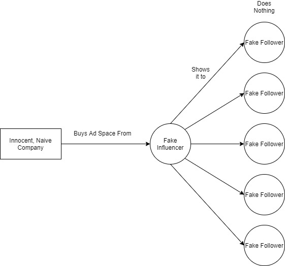
Let us look at social media, Instagram to be specific. It is an easy assumption that if you see an account being followed by millions of other accounts, that whoever owns this account must be something of a big deal <insert Anchorman gif>. Going the other way, even if someone didn’t have a lot of followers, but were followed by people whom had millions of followers themselves, then you could also assume that the former is a prominent individual to some capacity. This model could be translated to hubs and authorities from HITS.
It is not uncommon for people with large amounts of followers (authorities) to post advertisements on their accounts. Brands will partner with these authorities, called influencers, and pay them to run their ads running under the assumption that they are exposing their product or service to a large amount of people. But this may not be the case. It is a common practice for individuals on Instragram to purchase fake followers to make themselves look more important. So if a company were to run an ad through a fake influencer, all they are really doing is wasting their money as fake followers would not act on any advertisements. A report by Cheq, a cybersecurity company, has come to the conclusion that of the $8.5 billion spent on avertisements through influencers every year, about $1.3 billion is waster on fake influencers.
As time goes on, brands are becoming more cautious with how they select influencers to work with. In recent years, they have begun using tools to analyze how influencers get followers and who these followers are. What I think is really interesting, is that one of the red flags for a fake follower is when they follow thousands of people, which under HITS would give them a high hub score, but in this application, it should lower their value instead due to the high likelihood of them being fake. In addition to follower and following counts, the algorithms look at other factors including frequency of activity such as likes and posts.
While link analysis can be effective in numerous situations, without any aspect of quality included in, it may be difficult to apply correctly in other situations. I think that it isn’t out of the question to calculate a quality score for each node and use it as a factor in determining the authority and hub values. Given, this would be difficult and impractical using standard algorithms.
The Art of War was written by a Chinese ancient military strategist called Sun Tzu in late Spring and Autumn Period, it presents a lot of strategies of winning a war or battle and some of the aspects have a great influence on military planning even till now. The main idea about The Art of War is decision making and try to predict the opponent’s actions and then make the choice to dominant the war, which is the same as the game theory. However, the game theory is more about a mathematical approach of decision making, while The Art of War is more complicated than the game theory as it also considers human psychology facts and the situation under The Art of War is arguing is very fast changing (because anything could happen during a war) and there are too many unknown facts to do a mathematical calculation.
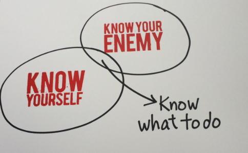
“If
you know both yourself and your enemy, you can win numerous (literally, “a
hundred”) battles without jeopardy” by The Art of War. It sates if someone
knows the opponents quite well, then they can predict what are the possible
actions that opponents will take so that they can come up with a solution to
win the battle.
This idea is similar to the game theory
as they all want to figure out a dominant way to win the game. The game theory
is built on all of the people will make the rational decisions and find all the
possible solutions and calculate the how many chances they could win and the
choose the best one. However, the “enemy” talked by Sun Tzu is way more complicated,
because Sun also considers the psychology
of the opponents, for example, the fear. During the war, if you let your enemy
fear about you, then there will a lager chance you can win it (during the cold
weapon era, bluffing is a common strategy as it will make the enemies think you
are strong, it is more like a deception, but in The Art of War, Sun states all the
warfare is based on deception).
The
reason I would like to talk about The Art of War is it is very impressive that
Sun Tzu camp up the ideas about handling the conflicts and wining a war is
really close to the game theory and written into book over 2500 years ago, even
though Sun Tzu did not know game theory at that time, but he really contributes
a great work to the world. The strategies Sun talks about not only can be
applied to military strategies studies but also for the business (as the
business is the modern warfare now).
In general,
the game theory and The Art of War can be applied to military strategy and some
other fields such as economy. The game theory is more like a mathematical way
to calculate the possibility of winning based on a stable and simple situation.
While The Art of War cannot calculated the possibility as the situation is way
more complex and not stable.
So far in our lectures, our understanding of Nash Equilibrium is the solution(s) which are the best responses to all other rational players, where no one can gain by unilaterally changing their response. This makes sense when we take a look at how game theory is applied to simple games – either rock paper scissors, prisoner’s dilemma, and so on. However, life is often far more complex and nuanced than our simple games can model – there are consequences, costs and requirements associated with each decision, and the outcome must be weighed against these costs. It’s not as simple as a win, or lose, and the cost of choosing different responses must factor into how we evaluate the best response to any situation. It is this belief that drove Basilio Gentile, Dario Paccagnan, Bolutife Ogunsula, and John Lygeros – postdoctoral researchers at ETH Zürich – to develop a new model of equilibriums, which factor in the cost of changing actions, which they call the Inertial Nash Equilibrium.
The authors of the paper published in October 2019, titled “The Nash Equilibrium with Inertia in Population Games” describe that applying an inertial model to population games helps generate new understandings of how actors respond to a set of choices. Specifically, they mention that in real life, a set of consequences – monetary, physical, specific limitations, etc. place a “cost” on response changes by the actors. The key insight that they provide for this is the fact that:
“introducing such costs leads to a larger set of equilibria that is in general not convex, even if the set of Nash equilibria without switching costs is so.”
– pg 1, Gentile et al.
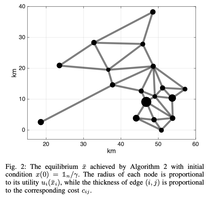
I chose this paper because I think it provides a novel idea regarding how we can model population games using game theory concepts. The paper provides numerous examples on how weighted and inertial models of these games lead to interesting analysis – particularly how ride-sharing (Uber, Lyft) drivers disperse themselves throughout metropolitan cities as a function of other drivers (basic Nash Equilibrium), but also as a function of average ride distance, gas cost, speed limits, and more (inertia, getting from one location to the next for ‘better’ ridership incurs cost to the driver, which plays a factor in their decision to stay put).
I found this article particularly interesting due to how it relates well to the content we cover in class pertaining to games, mixed-responses, pure responses, and Nash Equilibriums. We cover a lot of examples of the applications of Social Information Networks and network analysis, so I figured that sharing some of the applications of augmented Nash equilibriums could be interesting too. By introducing the concept of inertia and cost to moves, actors have additional considerations regarding what a Best response may be, which influences what unilateral moves make sense for them to consider. For interested readers that want to learn more about how this affects various topics, particularly ridesharing, please feel free to read the full paper here: https://arxiv.org/pdf/1910.00220.pdf
An example of how inertia and cost is applied to a game to model inertial Nash Equilibrium (2019)
Reference:
Basilio, G. (2019, October 1). The Nash Equilibrium with Inertia in Population Games. Retrieved November 6, 2019, from https://arxiv.org/pdf/1910.00220.pdf.
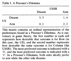
The Prisoner’s Dilemma can be explored throughout many historical conflicts. The concept can apply to a large range of scenarios, from small personal decisions to massive world wars.
A prime example of the Prisoner’s Dilemma can be seen during the Cold War between the United States and the Soviet Union. The Cold War was a nuclear arms race between the two opposing factions. Each country had two options: to arm or disarm their nuclear weapons. The possible outcomes of these choices between the United States and the Soviet Union is displayed by the following table:
It is easy to observe that it is a strictly dominant strategy for both parties to arm their nuclear weapons, because it would result in the best outcome for both choices of the opposing party. This is intuitive, because if, for example, if the United States arms their nuclear weapons, then it would be in the Soviet Union’s best interests to match their opponent’s military strength and also arm their weapons, in order to avoid annihilation and gain the opportunity to counterattack. In the other scenario, where the United States disarms their weapons, then the Soviet Union would be inclined to arm their weapons for military superiority. In both cases, arming is the better choice. The same mirrored argument applies to the United States reacting to the Soviet Union. Naturally, both countries chose to arm their weapons, and this large-scale application of the Prisoner’s Dilemma became known as the Cold War.
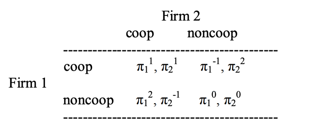
Shopping for groceries is an extremely common practice that we go through multiple times a month. It is important that we find local grocery stores that are cheap to make our trips inexpensive. But, due to the low amount of competition in the industry, these retailers take advantage of the consumers by pricing items approximately the same in order to control the market and increase their profit. There are a lot of factors that goes into deciding how to price items to gain the maximum profit possible but Ezeala-Harrison and Baffoe-Bonnie both show that given two retail stores that belong in a regional oligopoly (few competition), if they both operated as rivals, the best choice for both of the stores would be to not co-operate with each other.
Consider the following payoff matrix:
We will define “cooperate” as a store not playing any aggressive moves and “non-cooperate” as a store that is making aggressive decisions such as significantly altering prices of products that also belong to rivals. Considering the figure above, we can look at the power of each term to determine the payoff that the specific firm will receive (i.e power of 0 indicates breaking even while greater than 0 implies profit and less than 0 implies losing money). By observing the above figure, we can see that the Nash equilibrium of the decisions of these two firms is if they both do not co operate, implying a competitive environment where both stores are making aggressive actions. In the published paper, Ezeala-Harrison and Baffoe-Bonnie compute by probability, the best choice of both the firms which also concludes that both firms can establish greater benefits by not cooperating.
By our results of the payoff matrix above, we would expect that both firms that belong in an oligopoly would compete against each other aggressively, as it would give better results. In real life, this isn’t the case. There can be multiple reasons why the conclusions from the payoff matrix isn’t accurate (i.e various factors that go into choosing pricing for products) but the most likely cases are either 1) firms price match each other or 2) collusion between these firms. In an oligopoly market, the small amount of competition are given the opportunity to work together (sometimes illegally) in order to benefit all competition. This can involve both firms raising prices of the exact same products, leaving consumers no choice but to buy unreasonably priced groceries.
In conclusion, oligopoly markets involving the retail grocery industry exhibits behaviour that is not natural based on a simple Prisoners Dilemma model and indicates to us that price matching may occur between the firms in these markets or collusion with the stores exists. Either way, the local consumers unfortunately have to suffer consequences of buying overpriced products if they happen to live in regions dominated by few competition.
Reference
Ezeala-Harrison, F., & Baffoe-Bonnie, J. (2016, January 30). Market Concentration in the Grocery Retail Industry: Application of the Basic Prisoners’ Dilemma Model. Retrieved from http://www.scienpress.com/Upload/AMAE/Vol%206_1_3.pdf.
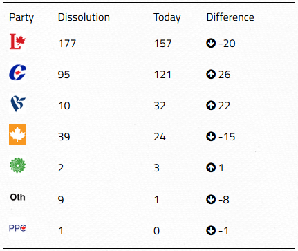
The recent Canadian Federal Election is an excellent example of the Balance Theorem at work, that is networks either contain only positive edges, or they are split into two factions. In Canadian Politics, this can be essentially seen as the Liberal vs Conservative divide with over 80% of the seats going to either the Liberal party or the Conservative party.
This split is not just limited to election results, our day to day lives exhibits this also. We tend to listen to those who form similar opinions with us and ignore or distance ourselves with those who disagree with us. This naturally leads to the state where each person is surrounded only with those they agree with, factions as seen in the Balance Theorem.
Ever wonder what it would be like to be related to royalty of ancient times past? What if I told you that if you’re European, then you’re related to King Charlemagne? Seems crazy, right? Well, lets examine an arbitrary person’s family tree. It would start with the person themselves, their 2 parents, 4 grand parents, etc… and resemble a complete binary tree. But if we think about this for a bit, we see that there is a bit of a contradiction. Going 30 generations back, so approximately 600 years if we assume a generation is approximately 20 years, a person would have 2^30 = 1,073,741,824 ancestors in that generation. But hold on! That is more than the number of people that would be alive in the whole world at that time, so what’s going on?
It turns out that our family trees aren’t just simple complete binary trees. The explanation lies in the fact that our family tree doesn’t have all unique ancestors, some ancestors take up multiple spots on the tree. This happens when parents of an ancestor are (knowingly or unknowingly) related to each other, which collapses the two parents’ family trees into a single tree.
This is known as pedigree collapse. After considering this, our family tree turns out to be a directed acyclic graph, since an individual cannot be their own ancestor, and a single ancestor can have multiple paths to the individual. How does this relate to King Charlemagne? Considering he lived from the years 742-814, there would have to have been a lot of pedigree collapse since no one individual could have distinct ancestors from those years until now. It was shown in 2013 by geneticists Peter Ralph and Graham Coop that all Europeans have the same common ancestors, going back around 1000 years. Thus all Europeans are related to King Charlemagne! Not only that, go back far enough and it is very likely that everyone is in some way related. It begs the question of how many degrees of separation there are between two individuals through their ancestry.
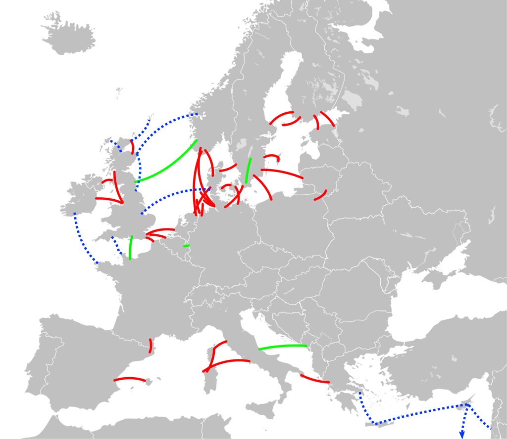
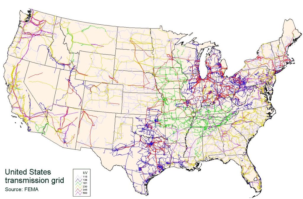
Countless device in our dailies lives use electricity. This number continues to increase as time passes by. To power these new devices we need ever more energy. The main source of electricity for the majority of devices is from a power grid. These massive physical networks can span across different countries and provide electricity for the majority of the world.
For a graph of a power grid we can take the … to be nodes and the cables between them to be edges. We can also measure the electrical current through an edge as the weight of that edge. We can use graph flow methods to measure the importance of different edges, and asses whether the given infrastructure is enough to handle the load. Occasionally there can be blackouts, which can occur as the result of some edge between two nodes being removed. Larger blackout can occur as the result of cascading failures occurring after several edges fail. These failures can result in increased flow on several edges, which may lead to these edges failing as well increasing the size of the blackout.


