Blizzard has been a mainstay in the video game industry for 19
years creating games which were massive successes and which have spanned
through generations including titles such as Warcraft, Diablo, Hearthstone, and
most recently Overwatch. Although Blizzard Entertainment has been a giant in
the video game industry for 19 years, the company has not held a spotless track
record, and the company is continuing to add blemishes to their reputation as
time goes on.
Earlier this October, controversy struck as Blizzard disciplined a player for speaking up on the recent political events happening in Hong Kong. During a tournament, a player was interviewed after a match and brought awareness to the Hong Kong protests by donning a ski mask and gas mask and stated “Liberate Hong Kong. Revolution of our age.” This put Blizzard Entertainment in a difficult position due to their ties with China as Tencent, a giant in the Chinese gaming industry, owns a stake in Blizzard and the relations between China and Hong Kong are obviously not great at the moment. Blizzard responded with a harsh disciplinary action of removing all earnings from the player, as well as banning the player for a whole year. Additionally, Blizzard punished the two commentators giving the interview by immediately dismissing both of them. This has led to an uproar within the community against Blizzard for their actions which draws a parallel to the Balance Theorem.
Prior to all of the controversy and prior to the political
disagreements between China and Hong Kong there was relative balance between
Blizzard, China, Hong Kong, as well as the community. If represented by a
signed graph, it would be a complete signed graph with only positive edges.
However, China and Hong Kong has had conflicts between each other which
disrupted the balance between the four parties. This has led to the divide
where Blizzard sided with China and the community siding with Hong Kong to form
two parties and it has partitioned the group.
However, Blizzard has recently taken a step back on the disciplinary actions on both the player and both commentators so it remains to be seen if the parties involved will in fact make peace with one another or if there will be a permanent divide caused.
Social media has change the way we all interact with each other across the world. It can be many different types of media from text to image, and even touch. It can also cover many different ranges from across the world to you’re friend sitting next to you. This flexibility is one of the traits which gives social media this appeal as it creates a piece of the internet for everyone.
The internet was initially created without security in mind – internet was a better place, it was a simplier place. As the internet grew, malicious intent grew through virus and exploits which resulted in countermeasures such as encryption. Malicious intent can be “physical” like DOS attacks and leaking of passwords, but it can also be social like astroturfing attacks.
The acts of astroturfing vs real widespread movement represented by real grass and artifical turf
Astroturfing is “the attempt to create an impression of widespread grassroots support for a policy, individual, or product, where little such support exists”. In layman’s terms, we are creating a “movement” for something through the seeding from a mass of people. The attack is similar to DOS, where a set of hacked or created accounts are used to post about a certain topic. It is becoming a very widespread and effective means of advertisement, but manipulates the social media leading to skewed impressions and misrepresentations.
Relating this back to graph theory, using graphs to represent different characteristics we are able to visualize relationships between these astrobots. In the diagram below, the edges represent a keyword relationship between astrobots, which are nodes. From this picture, we can see different communities from the clusters with represent different types of account, such as suspended accounts, used to as a bot. By using a signed colored graph, where a positive sign is given to nodes of a similar type and negative otherwise, we are able to develop communities in relationship the keyword attacks.
Graph representing the relationship between astrobots via attacking the same keyword on the same day
Countering astrobots can be a very hairy situation, since depending on the type of bot, there can be side-effects from actions such as suspsension and/or banning. For example, these bots can be affected without the user’s acknowledgement, therefore suspension would led to anger or fustration from the original owner. By using graph theory, we are able to learn about the motives and characteristics of astrobots from different perspectives. Using this information, we are able to prevent this from happening and apply the most appropriate action without affecting actual users.
References
Elmas, Tuğrulcan, et al. “Lateral Astroturfing Attacks on Twitter Trending Topics.” ArXiv.org, 17 Oct. 2019, https://arxiv.org/pdf/1910.07783.pdf.
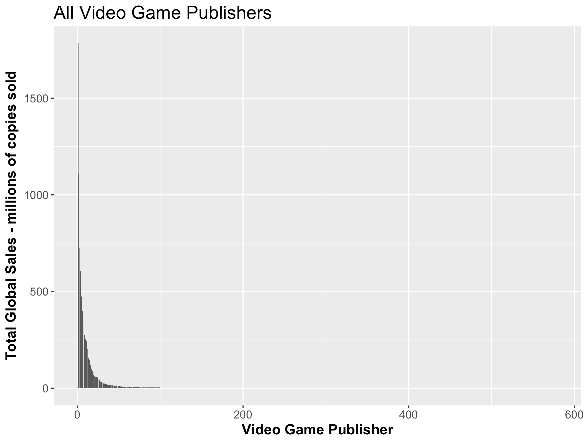
An interesting article posted in June of 2018 indicates that the power law can be observed in a number of forms of media, with some displaying a steeper curve than others. It is interesting to observe these distributions that can be modelled with math exist in the real world. For example, observe how steep the graph showing success of video game publishers is:
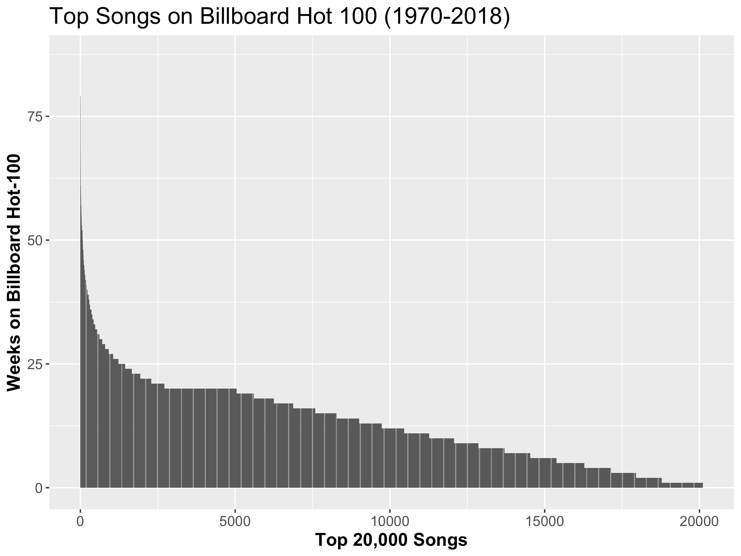
The success of video game publishers is measured by their total global sales, and it is clear that that a select few have lots of success while the rest have very little. In comparison, other forms of media are not as punishing to those less successful, like with song artists:
The curve here is far less steep, indicating that it is easier to get one of your songs to stay on the Billboard Hot-100 for a couple weeks than it is to be a successful video game publisher.
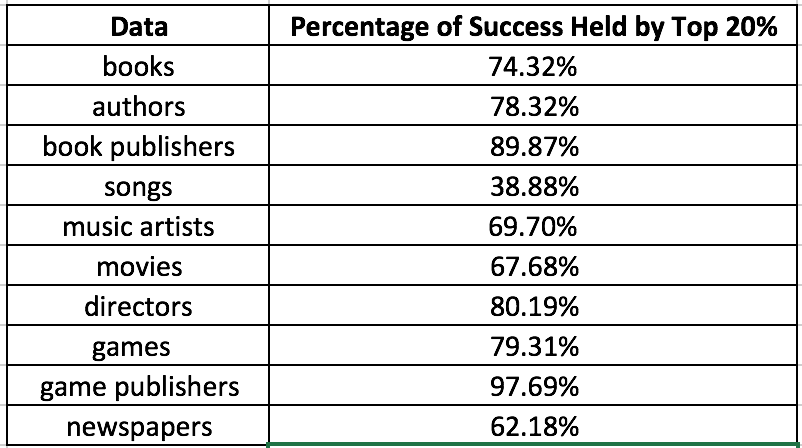
The article also discusses the 80-20 rule, also knows as the Pareto Principle, and looks at how much success the top 20% of entries for each industry have.
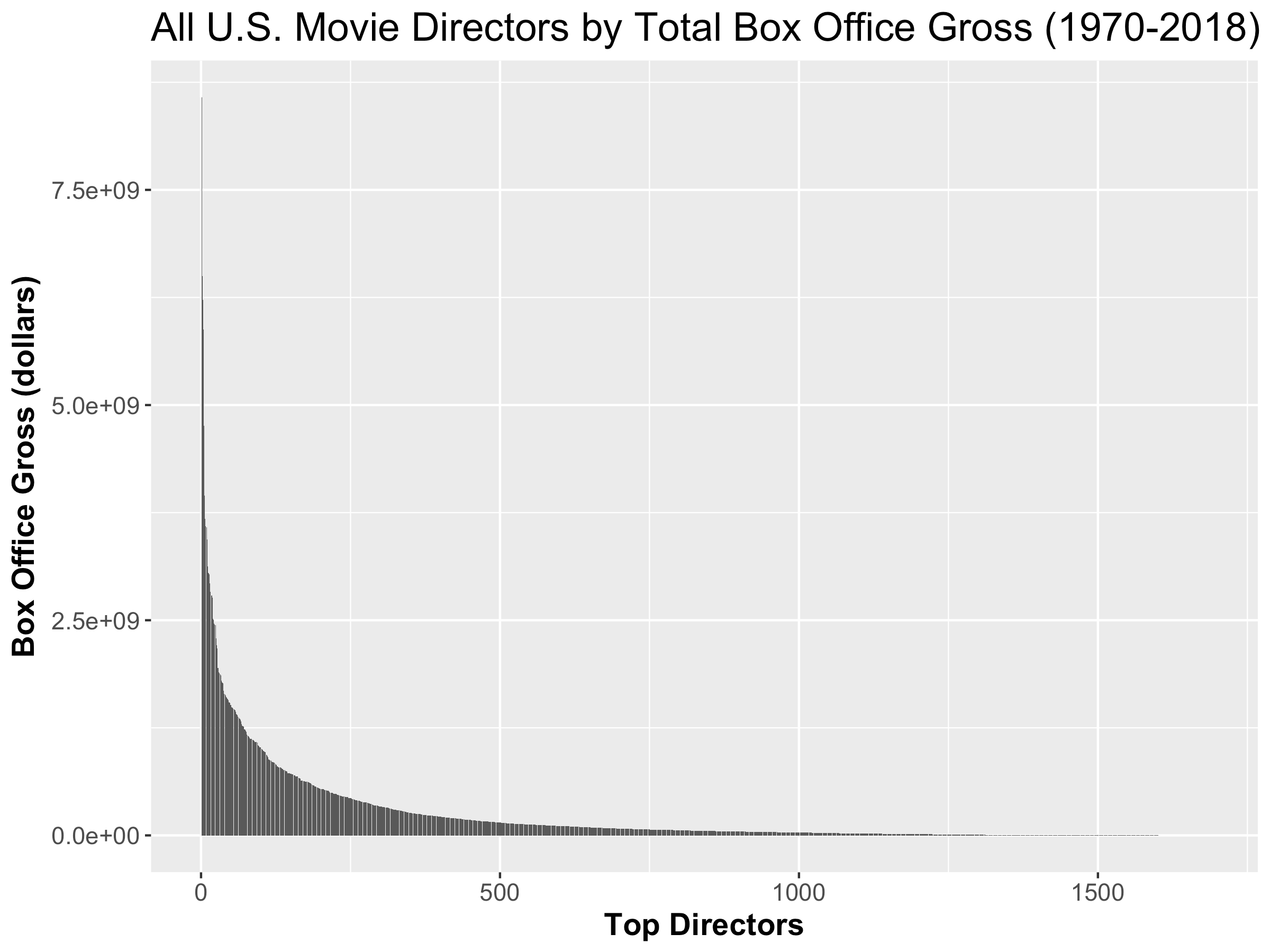
It should be noticed that these numbers are related to the steepness of the graph, as one can see that the top 20% of game publishers own 97.69% of all the success in the industry, hence the extremely steep curve. On the other hand, the top 20% of songs only hold 38.88% of the overall song success. It was no accident that I chose those two specific charts earlier in the article. In fact, the tail of the songs chart actually does not follow the power law, which make it even more interesting that out of all the forms of measuring success in the media industry, the number of weeks a song stays on the Billboard Hot-100 is the only one to not follow the power law distribution. Some industries also follow the 80-20 rule very closely, such as success of movie directors:
This curve looks far more like what I expect to see when I think of the power law.
This obviously relates to the entire discussion of the power law from lecture as well as whether or not success depends on simply being lucky or being first, as the information above would suggest that early success is very important in the world of media, although less important for songs than it is for video game publishers.
I chose to write about this article because most of what we see in today’s world is a product of the media industry, and so I thought it was interesting to see how closely success in this industry follows the power law distribution, as likely no movie director or book author is thinking about it when creating their work, and yet it shows up anyways. We were shown an example of this in class with the experiment carried out, but this is a far more recent look of the topic, and I thought it was worthwhile to post.
“We cannot stop natural disasters but we can arm ourselves with knowledge: so many lives wouldn’t have to be lost if there was enough disaster preparedness.” – Petra Nemcova (4)
The world has finally begun to act in preventing climate change. Unfortunately, the damage has already been done, and what are defined as natural disasters have seen a dramatic increase within the past 50 or so years (1).
Something that I know for a fact I take for granted, and I’m sure many others do as well, is our infrastructure that we have within Toronto. Such infrastructure includes: our road systems, power grid, drainage systems, sewage system, internet lines, and many more. Thankfully, Toronto is situated in a very key geological region where we do not see many natural disasters such as hurricanes, floods, or forest fires; but many highly densely populated areas of the world are in these danger zones (2).
One of the reasons as to why these disasters can become so catastrophic in terms of monetary damage, and for the local population, is due to the effects that they have on the local infrastructure. There are times when even a failure of a key piece of infrastructure can cause such an event – such as a dam breaking (3). Without access to this infrastructure, locals are unable to deliver aid to the afflicted, or even worse, notify residents of certain events that can put them in danger or affect them in some way.
Thankfully, the local population usually has some kind of remediation plan set in place that would help mitigate the damage. Although these infrastructure systems are built to be resilient, they are not immune.
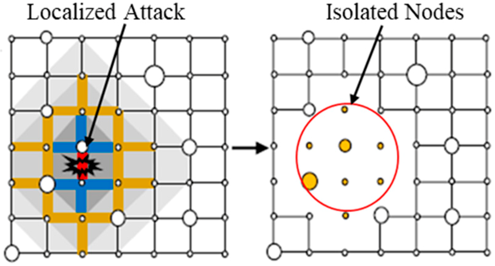
How does any of this relate back to what we’ve been discussing within CSCC46 you may ask yourself? As we’ve already explored, infrastructures such as the internet can be treated as a network. I will now introduce a network that has not yet been covered by the course: a lattice network. You may think of it as a matrix where each index is a node that has edges connecting to its direct index neighbours, as well as, the index one level above and one level below. In mathematical terms we can conceptualize this as the following: For a given nxn matrix A, an index a_(i,j) has an edge to the following set {a_(i, j – 1), a_(i, j + 1), a_(i + 1, j), a_(i – 1, j)}. Back to the original question, many infrastructure systems can be plotted using such a lattice network, think of road systems, sewage systems, or power grids as examples.
When speaking about such a lattice network, a natural disaster has the capability of breaking such a lattice structure, thus disabling the local infrastructure. Such an event is called a localized attack. I came across a very interesting article (Inspiration) that explored recovery assessments of such networked infrastructure under such an attack. Understanding the best way – in terms of efficiency, cost, and possibly human lives – to repair such a network can prove to be quite useful when it comes to planning ahead. This ‘best way’ is what is referred to as resilience.
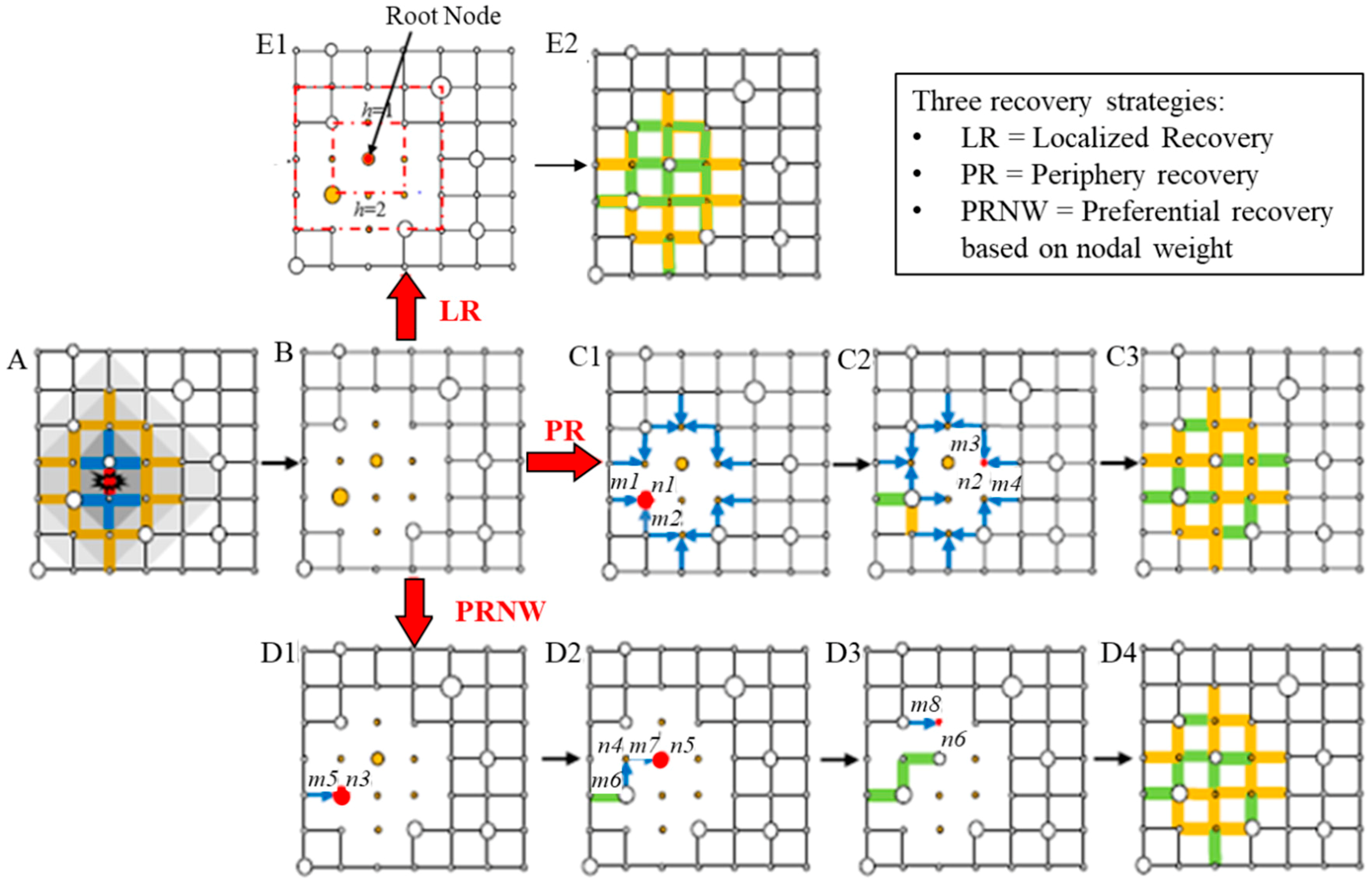
The article explores different recovery strategies that would be able to recover from such an event, as demonstrated in the image below. The Periphery Recovery strategy targets the most populous nodes – in terms of people served – before going to repair the attacked node – we will call this the root node. The Preferential Recovery strategy targets nodes that that have edges leading to the most populous nodes. And lastly, the Localized Recovery strategy that assigns a certain max weight w to the root node, and then some weight w – d where d is the distance away from the root node and basically works in a Dijkstras’ fashion to repair the root node as the target in hopes of restoring the full network.
The article further explores something called the resilience metricΦ which is used to analyze the resilience of a network given some localized attack and can be used to create a resilience-based optimization model – using the strategies listed above – in comparison to some existing network.
An example was given where a water distribution system was used to demonstrate such an analysis. Meant to stop propagation of issues resulting from the failure of the water distribution shortage and to bring back the system in the most efficient way to ensure its resilience is maximized.
I won’t bore you with the math, but this was simply a small look at the potential that network analysis can have to strengthen existing infrastructure and understand how to maximize it’s resilience towards localized attacks which can be the difference between life and death during a natural disaster.
I end this blog post with some parting thoughts. Our infrastructure that we’ve put in place is responsible for getting you your water, your heat, your electricity, that most of us take for granted. If such a localized attack were to occur as result of a natural disaster, or other means, our number one priority should be in restoring this network to ensure it has no further cascading negative effects on it’s populous.
Inspiration: Afrin, T., & Yodo, N. (2019). Resilience-Based Recovery Assessments of Networked Infrastructure Systems under Localized Attacks. Infrastructures, 4(1), 11.
Citations:
Hannah Ritchie and Max Roser (2019) – “Natural Disasters”. Published online at OurWorldInData.org. Retrieved from https://ourworldindata.org/natural-disasters
Dillinger, Jessica. (2018, September 26). Countries Most Prone to Natural Disasters. Retrieved from https://www.worldatlas.com/articles/countries-with-the-deadliest-natural-disasters.html
CNN Wire Staff. (2010, July 24). Dam fails in eastern Iowa, causing massive flooding. Retrieved from http://www.cnn.com/2010/US/07/24/iowa.dam.breach/index.html
Petra Nemcova Quotes. (n.d.). BrainyQuote.com. Retrieved October 24, 2019, from BrainyQuote.com Web site: https://www.brainyquote.com/quotes/petra_nemcova_426837
FC Barcelona is a well known soccer club which plays in the Spanish League La Liga and during the 2009-2010 season they were unbeatable winning six major championships. You might wonder what their secret to success was during that season and if it is possible to analyze the aspects of their game better than existing methods. Can we analyze this using networks and concepts learnt in CSCC46? A recent study from Universidad Rey Juan Carlos proves that through using networks and analyzing it is possible to better understand the style of play.
First a network was created with nodes representing players in a particular game and an edge between each player existed if there was a pass between them at any time. The study also recorded the position of each player during the game. The network also contained a sliding window of 50 passes which will delete the very first edge as the game progresses and this helped in analysing different phases of the game.
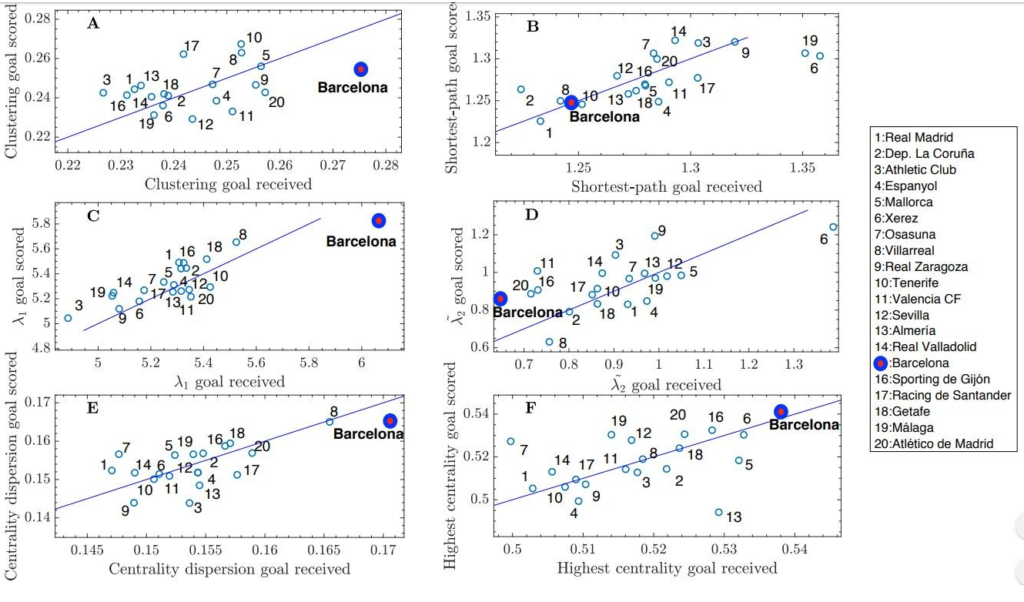
What did this network reveal about the team? The network showed central team players through which the ball frequently passes through , triads between players who frequently passed the ball between each other and more. Calculating the clustering coefficient of this network concluded that Barcelona had one of best passing between neighbours of its players among all teams. It was also decided that Barcelona had the best shortest average paths which again shows the skill of passing across the team. The study also predicted probabilities of the team scoring a goal given a particular network.
Here is a graph that shows properties of the network from the study.
It is interesting how a network of a sports team can reveal a lot more about the style of a team and I wonder what the potential uses of it are in the future. Maybe opposing team coaches can use this information to better tackle a strong team or to use some of the techniques and strategies in their own team to improve.
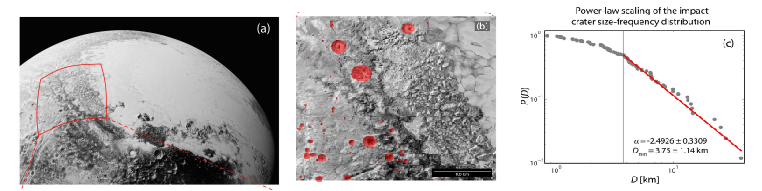
The existence of the power law has been witnessed in various networks created by humans in various forms as discussed in class. As previously discussed it shows in various social constructs such as social networks and even actor collaborations, however the power law also makes itself apparent within nature and in our planet. What is even more interesting however, is that the power law exists to even a scale as large as celestial bodies, from Pluto, to our moon and even the sun itself, the power law is everywhere.
One study looks into the the craters in Pluto, upon the recent high resolution pictures of Pluto, scientists were able to look at the actual craters in the planet. It investigated 87 craters in Pluto, ranging from sizes of 0.87km to 37.77km. It was found that there was a scaling coefficient of “α = −2.4926 ± 0.3309”, with a “Dmin = 3.75 ± 1.14 km” (or xmin if we use the formula we discussed in class). Upon values of distance D within the range “[3.75 ± 1.14 km, 37.77 km]” there was a log likelihood (L) = 104.5688. It is incredibly interesting that these scientists are using the same formulas we are to calculate the scale and witness power law on a celestial scale!
Below indicates a segment of craters within Pluto that were analyzed for their crater size
The study then continued to look at how these craters were very comparable to power-laws in other celestial bodies such as our Moon, Mar’s satellites Phobos and Deimos, and even the Earth! As an interesting tangent, the study also referenced how the power law existed in the relationship between the frequency of solar flares and total flare energy. Going on to provide other examples such as the distribution of initial masses for star populations, Kepler’s third law, and even to the scale of the distribution of galaxies in the universe! It is incredible to think of how this law shows itself throughout the universe. From human social constructs, things we made, to the scale of galaxies in the Universe!
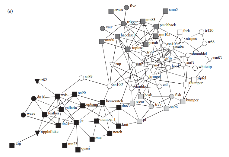
You’ve might have read articles on the news or blogs about how dolphins are very similar to humans and they way they behave. Dolphins have a naturally friendly relationship with humans and many dolphins and human interactions have been amiable. Given their social aptitudes, many have wondered how they interact with each other. Dolphins can form friendships and form their own social networks in which they find comfort associating within. This also brings up the social hierarchy in the roles that each dolphin plays in their social circle and where each dolphin fits in within their miniature society. While dolphins can’t come in to do interviews or fill out surveys, David Lusseau and M. E. J. Newman analyzed these relationships to find measures of association and behavior of a group of bottle-nose dolphins in New Zealand.
HTWD1X Bottlenose Dolphin (Tursiops Truncates)
Lusseau and Newman started by determining the communities and modeled a graph of betweeness of an assemble of dolphins through Girvan Newman and then identifying the critical dolphins that keep the community together, and the result of these groupings that create homophily within the entire group structure. While the analysis of humans brings upon many concrete statistics that can be compared such as age, race, gender, occupation, etc, dolphin can only be measured in age (which was mostly estimated) and gender (which was observed).
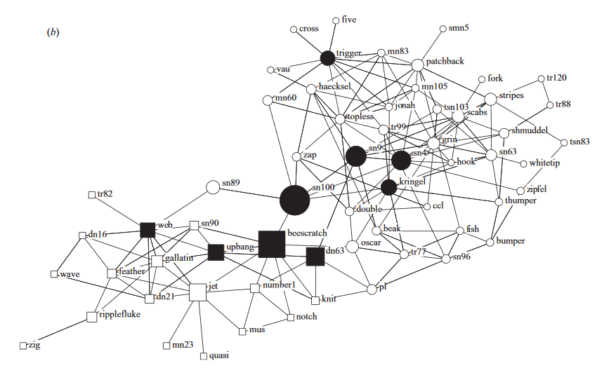
This is their findings presented through a Girvan and Newman algorithm, finding and identifying communities. Males are represented as squares while females are circles. Ones that could not have their gender identified are triangles. In this diagram, they concluded that there 2 major communities, with 1 split into 3 sub communities. The black shaded group forms one community while all other nodes form another, splitting between smaller sub communities that interact within the their own group more frequently.
This graph shows the dolphins that the center of these communities and have a betweeness greater than 7.33 . These dolphins marked by the filled in shapes are the “brokers” between communities that will interact with other communities as well. They found that when sn100 was away, the 2 communities almost never interacted and drove the 2 groups apart.
We can see that even dolphins have exhibit homophily and will stick within their own group of friends when presented and it is interesting to see how close dolphins and us are alike.
References
Lusseau, D., & Newman, M. E. J. (n.d.). Identifying the role thatanimals play in their socialnetworks. Retrieved October 23, 2019, from https://www.ncbi.nlm.nih.gov/pmc/articles/PMC1810112/pdf/15801609.pdf.
Have you ever had one guy throwing your match in that MOBA (multiplayer online battle arena) game, FPS (first person shooter), or other game? A lot of the time I certainly had this occur, and its not fun. Sometimes, when matched up with teammates of similar skill as well as opponents of similar skill, these result in the best possible matches you can have as things get super close. Zhenxing Chen, a researcher at Northeastern University, has created a matchmaking algorithm that uses familiar items we have learned in class.
The algorithm begins by taking all other players in the que and puts them into a complete graph. Each edge has what is called a “churn” rating. Essentially, this is measured by how much time has elapsed since the last matchmaking decision was made and the time elapsed before the player chose to play the game again. Players are matched by attempting to pair the minimum sum of edges.
This model focuses on maximizing player engagement, rather than on player skill like other matchmaking systems including the “Bradley-Terry” model or the “elo” model. While this may cause some more imbalance in terms of player skill for matchmaking, this model will result in more player engagement, and therefore more player retention.
A phrase commonly used in MOBAs for someone who really wants to play mid
But how do we measure player engagement correctly? Some factors that we can say for sure are both time spent playing and/or money spent playing the game. Additionally, as discussed above, time between sessions can also be a good factor. If a player had a very poor matchmaking experience, this makes it more likely that they will want to quit the game or take a long break from it. However, good matchmaking experiences will make players want to play more, therefore resulting in a shorter time period between matchmaking processes.
There where a few very interesting finds when experimenting with this algorithm. For the scenario of a players total wins plus the total amount of losses is greater than two times the amount of draws, then our engagement matchmaking algorithm is approximately equal to the skill based models discussed previously. However, if it is less than rather than greater than, then skill based matchmaking ends up being the worst form of matchmaking.
When testing out the engagement matchmaking algorithm, it was tested with a random sample of players between 100 to 500 in size. The matchmaking systems used were worst matchmaking, skill based matchmaking, random matchmaking, and our engagement matchmaking. The engagement matchmaking managed to have slightly higher player retention than all the other forms of matchmaking.
It is very cool to see how graphs can be used for video game matchmaking like this, especially when it is within your favorite hobby. Graphs can be very useful in the most unexpected ways!
Road networks are essential for transportation in many states, cities, towns, and villages. People travel on roads everyday in order to get to work, to school, to business meetings, to transport their goods, etc. A big problem in road networks is finding shortest paths between various locations. A motivating example of why we want to find shortest paths between various locations in road networks is google maps. Ever tried using google maps to get the fastest direction from your house to school? Google maps tries to find the shortest path that gets you there the fastest.
Shortest path problems are inevitable in road network applications such as city emergency handling and drive guide handling. I am going to look at how to tackle these problems, using graph theory which we learned in lecture to give a representation of the network and an efficient algorithm for finding shortest path from every node to every other node.
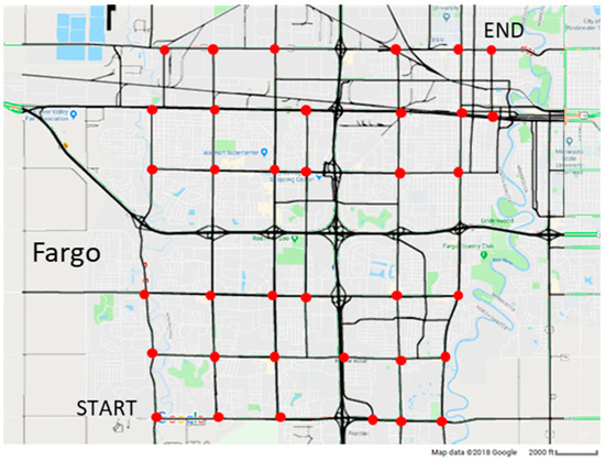
A way to tackle these shortest path problems in road networks is to use Dijkstra’s shortest path algorithm. Dijkstra’s Algorithm is a graph search algorithm that solves the single-source shortest path problem for a graph with non negative edge weight, producing a shortest path tree. For example, suppose the vertices of the graph are cities, the edges are direct roads, and the edge weights are driving distances between pairs of cities. Dijkstra’s algorithm can be used to find the shortest route between one city and all other cities.
The search space of Dijkstra’s algorithm on a road network, for a given source and target.
Dijkstra’s algorithm works as follows.
Step 1: Start at the ending vertex by marking it with a distance of 0, because it’s 0 units from the end. Call this vertex your current vertex, and put a circle around it indicating as such.
Step 2: Identify all of the vertices that are connected to the current vertex with an edge. Calculate their distance to the end by adding the weight of the edge to the mark on the current vertex. Mark each of the vertices with their corresponding distance, but only change a vertex’s mark if it’s less than a previous mark. Each time you mark the starting vertex with a mark, keep track of the path that resulted in that mark.
Step 3: Label the current vertex as visited by putting an X over it. Once a vertex is visited, we won’t look at it again.
Step 4: Of the vertices you just marked, find the one with the smallest mark, and make it your current vertex. Now, you can start again from step 2.
Step 5: Once you’ve labeled the beginning vertex as visited – stop. The distance of the shortest path is the mark of the starting vertex, and the shortest path is the path that resulted in that mark.
Dijkstra’s algorithm in stages. Highlighted green part is the nodes included at each step and the highlighted red edges are the shortest edges included in the algorithm for the tree.
Dijkstra’s algorithm provides us with a very efficient way to find shortest path. This algorithm is a very useful practical algorithm for finding shortest paths in road networks. Using graph theory, we can represent these road networks as vertices and edges, with edge weights, which gives us a representation of the networks in which we can use dijkstra’s algorithm to find the shortest path from a vertex to every other vertex.
As we have learned in class we can represent data in the form of networks which we can use to better understand systems. One such useful application of networks is in the analysis of how disease spreads among the population. One study from 2005 called “The Impacts of Network Topology on Disease Spread” uses various random networks to do just that.
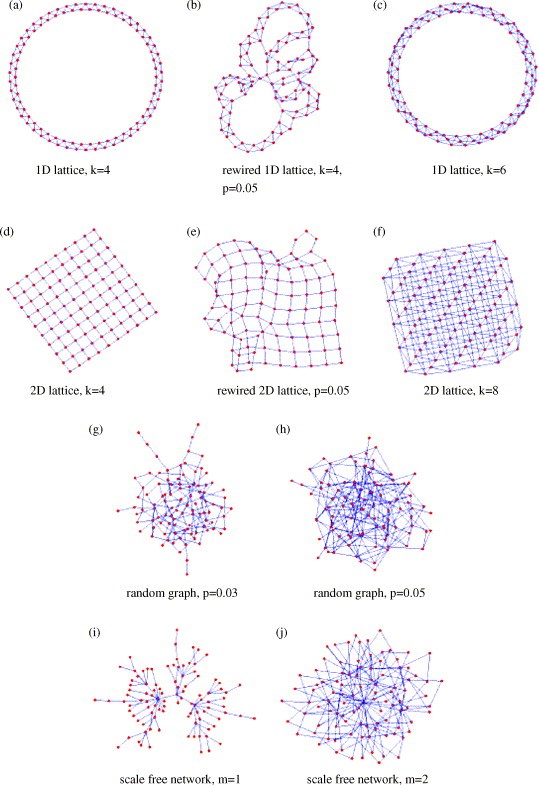
In the study it randomly generated four different types of networks of 500 nodes with similar amount of edges, but randomly assigned. The following types of networks were exactly like the ones we learned in class:
(i) – The Erdős–Rényi model (1960) which we learned in class as Gnp. As we know these random networks have low clustering coefficients and a binomial degree distribution.
(ii) – Regular lattices where each node is connect to k nearest neighbours to form either a grid of an array. These networks has a high clustering coefficient, but relatively high average path length since nodes only connect to their nearest neighbours.
(iii) – Rewired lattices (Watts-Strogatz 1998) where we start with a low-dimensional lattice (grid or array) and rewire to introduce randomness (“shortcuts”). By rewiring this introduces more clustering and short paths, thus lowering the average path length.
(iv) – Scale-free networks that have a power-law tail in their degree distribution. These networks have small average path lengths and low clustering.
The types of networks randomly generated in the simulation.
The following are the properties of the various networks randomly generated with a set amount of vertices (nodes) and similar amount of edges. It is interesting to note that the average path length.
Network type
n (vertices)
M (edges)
K (degree)
C (clustering)
D (length)
S (significance)
Random graph (RG)
500
1905 (33.9)
7.62 (2.71)
0.02 (0.00)
5.67 (2.19)
4.47 (0.25)
Scale-free network (SF)
500
1990
7.96 (8.18)
0.07 (0.00)
2.93
(0.02)
5.60 (0.04)
1D lattice (1D)
500
2000
8.00
0.64
31.69
1.39
2D lattice (2D)
500
1865
7.46
0.23
8.00
1.84
Rewired 1D lattice (1DR)
500
2000
8.00 (0.35)
0.62 (0.00)
8.19 (0.45)
1.59 (0.02)
Rewired 2D lattice (2DR)
500
1865
7.46 (0.33)
0.21 (0.00)
4.95 (0.05)
1.96 (0.01)
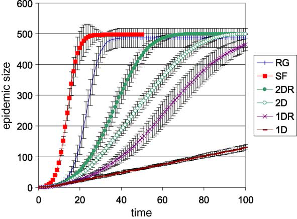
The nodes in these networks representing susceptible individuals to diseases and the edges representing a potential method of transmission for the disease. An infected node has a certain probability to infect all its neignbours after each time step. After a node infects another node, there is a time delay until that node becomes capable of infecting other nodes. Even after that, there is a time latency until an infected node becomes immune to the disease, thus non-infectious. Initially one node is infected in a network and the researchers analyzed how the disease spread through the network. They ran many simulations with varying infection probability on all of the types of graphs found that network types had an impact on how fast the epidemic spread. From fastest to slowest rate of infection:
Scale-free network
The Erdős–Rényi model (1960) (Gnp )
Rewired 2D lattice
2D lattice
Rewired 1D lattice
1D lattice
Visual graph showing how the epidemic spread for different networks. Probability of infection = 0.1, latent period = 2 time steps, infectious period = 10 time steps.
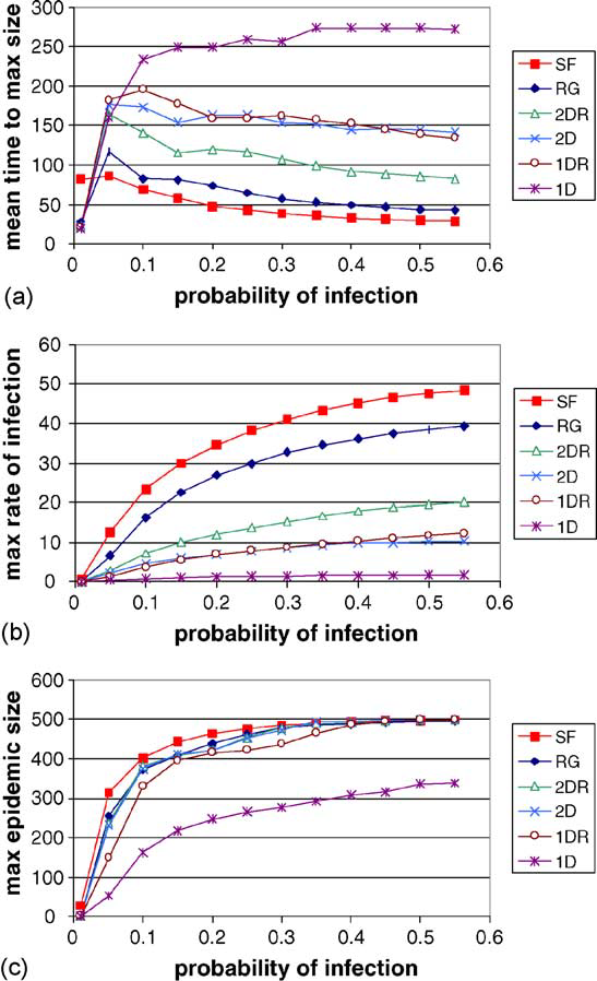
It is interesting to note that scale-free networks resulted in the largest epidemics for any level of infection. It reached the maximum epidemic size of 500 sooner than the other networks for any probability of infection. 1D lattices never reached the max epidemic size and grew linearly.
The averaged results from 10 simulated epidemics for each network.
It is important to ask why is it that epidemics spread quickly in scale-free networks but spread poorly in 1D lattice networks. The high average path length in 1D lattices and low average path length in scale-free networks helps explain that. In 1D lattices the high average path lengths prevents the infectious nodes from spreading the infection to distant clusters. The infection only grows outwards from the inital cluster. In scale-free networks, the low average path lengths enable infectious nodes to infect far away clusters which help quicken the spread of the infection. It now becomes clear why the rewired 2D lattice and rewired 1D lattice spread infections better than their non-rewired counterpart. The rewiring introduces more shortcut paths which lower the average path length which helps spread the infection faster.
Although the these were simulations on randomly generated networks, they show how understanding networks, random networks in this case, can help us understand real life problems.
References:
Shirley, Mark D.f., and Steve P. Rushton. “The Impacts of Network Topology on Disease Spread.” Ecological Complexity, vol. 2, no. 3, 2005, pp. 287–299., doi:10.1016/j.ecocom.2005.04.005.