Crowded Streets
With a population of almost 2.8 million in the city, not even accounting for those that commute daily for work, Toronto has to move a lot of people through a small space, fast. Car traffic through the city is slow at the best of times, and with alternative transportation becoming increasingly popular, models which can help predict movement through a city are increasingly valuable. When looking at how people get from point A to point B, pedestrian traffic seems a good place to start. Andres Sevtsuk mentions in their paper that increased pedestrian traffic is positively associated with the sustainability, health, and economic performance of a city, so there is likely to be interest in developments which promote walking in the future..
Betweenness is a clear choice for modelling this – for the most part, people tend to want to take short paths from their source to their destination, so by modelling locations as nodes and the paths between them as edges, we can predict the amount of traffic along an edge by calculating it’s flow. Unfortunately (for computer scientists, at least), not everyone takes the exact shortest path from every source to every destination, and not all locations are created equal. Because of this, a few modifications need to be made to the Girvan-Newman algorithm as described in lecture to more accurately represent this case.
Walking the Line
While this paper by Andres Sevtsuk chose Kendall Square in Cambridge to analyze, we will use a simplified example to demonstrate how the changes to the betweenness algorithm affect the distribution of flow. Let’s consider the following network:
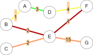
In the above graph, edges are coloured based on their betweenness, with green edges containing the least flow and red edges containing the most. Betweenness was calculated using the Girvan-Newmann algorithm with no special modifications. While this is a decent estimate, it assumes all nodes are equally desirable sources and destinations, and every traversed path will be optimal. Andres Sevtsuk proposes six changes to allow this calculation to better reflect actual walking patterns.
First, there is usually a defined source and destination during trips. For example, if it is around lunchtime and A, B, and C are all businesses or apartments, while F and G are restaurants, we expect more traffic along the paths to F and G. This is accompanied by a drop in the flow of edge (C, E), since not many people are walking to C.
Second, not many people are willing to walk several hours for lunch, and long paths are often undesirable. By implementing a ‘search radius’ we can define a maximum path length which limits flow to nodes which are too far away.
Third, the quickest path is not always the best. On busy days, travelers might opt to take the ‘scenic route’ from B to F through A, since it only incurs a path length of 7 instead of 6. To account for this, a ‘detour ratio’ is added, which allows flow to be split amongst ‘plausible’ paths with similar weights instead of just equal weights.
Fourth, some sources contain far more people than others. Suppose A is a high rise or large office, while B and C are small by comparison. In this case, most of the traffic will come from A, so nodes can be assigned a weight to represent this.
Fifth, sometimes the best option is simply the closest option. According to Andres, shorter trips are exponentially more likely than longer ones, so each destination is assigned a ‘destination elasticity’ term based on it’s weight and distance, which makes trips to it more likely.
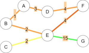
Finally, similar to above, sometimes one restaurant is simply better than it’s competition. By using a modified version of Huff’s model, the attractiveness of certain destinations can be accounted for so they are assigned more flow.
No Two Cities the Same
While the simple example illustrated above ended up largely homogenous in terms of flow, by varying the six parameters above drastically different graphs can be obtained. For example, if B produced the most traffic, C was now a destination, and pedestrians heavily favoured short trips, the graph may change to look like the following:
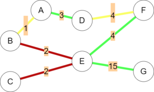
The advantage of using altered betweenness is the Girvan-Newman algorithm is very comprehensive by default – considering every possible combination of source and destination. This means it will easily detect the cumulative effects of multiple sources, even if low traffic is expected from them (for example, any pedestrians moving from A to F in the above graph). It is also very responsive to changes in parameters, taking into account every possible effect they have on a graph.
Hopefully, by applying this algorithm to prospective developments, city planners can work to make pathways which help foot traffic move more smoothly, and limit car traffic through high-flow areas to improve safety. Additionally, by altering some parameters such as search radius and destination elasticity, this model can be applied to other modes of transportation such as biking or driving, ensuring that no matter where or how you get lunch, you will never be seeing red.
References
Jones, R. P., & Ward, L (2022, October 5). Dangerous roads and slow progress: Road safety becomes issue on Toronto campaign trail. CBC News. https://www.cbc.ca/news/canada/toronto/toronto-election-vision-zero-1.6605819
(2021) Estimating Pedestrian Flows on Street Networks. Journal of the American Planning Association, 87(4), 512-526. DOI: 10.1080/01944363.2020.1864758
Statistics Canada. 2022. (table). Census Profile. 2021 Census of Population. Statistics Canada Catalogue no. 98-316-X2021001. Ottawa. Released September 21, 2022.
https://www12.statcan.gc.ca/census-recensement/2021/dp-pd/prof/index.cfm? (accessed October 7, 2022)