An invasive team sport is any sport where two opposing teams battle for space and score points within a given time frame. Soccer, hockey and basketball are just some examples of invasive sports. The similarity between these games allows data scientists to uncover patterns and develop analysis techniques that work for all of these games at once.
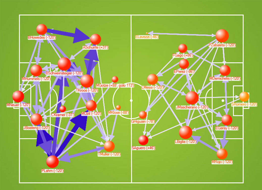
A graph like the one shown above is commonly used to represent invasive sports. In the simplest version, players are nodes and completed passes between players are directed weighted edges. This type of graph can tell us the most common passes and which players work together the most but it lacks depth in its information. Possession changes, shot attempts and shots scored are prominently missing from these graphs which create big gaps in data regarding a teams performance.
Temporal Bipartite Graphs
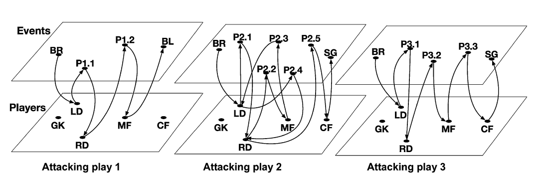
In an attempt to better understand offense, temporal bipartite graphs can be used to better represent attacking plays for invasive sports.
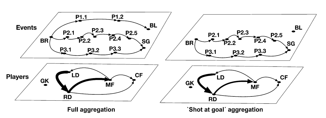
The bottom set of the graph contains nodes representing players, and the other set represents events such as passes, shot attempts etc.. A network like this should be created for each individual attacking play so an aggregation of all of these plays into one graph can be useful for analysis.
What can we learn?
Most interactive player:
The node with the highest degree represents the player who has had the most interactions (passes) during the game.
Intermediary players:
The node with the largest betweenness value will show us which player is present in the most shortest paths between other players. This metric is not directly useful because the shortest path is not necessarily the one taken when a goal is scored.
Team’s pace:
By counting the number of nodes in each attacking play we can tell how fast or slow a team executes their attacking plays and see their style. Does a star player hold possession disproportionally? Is the team particularly good with fast breaks or slower plays?
Best supporting player:
Calculating the eigenvector centrality of the player nodes, we can see who is the most depended on during attacking plays. This statistic is calculated based on a nodes degree and the degree of its neighbors. The player that tops this metric is quite central to a teams offense.
Clusters within the team:
We can calculate the clustering coefficient for each of the players as well. This will show us which players act as a middle man in the offensive structure of the team.
Along with this we can see if there exists triadic closures which indicate that 3 players have worked together during an attacking play.
Conclusion
Note that all the data collected for this offensive analysis would be useful for construction or criticism a defensive playbook as well. We could simply compute the same data for opposing teams offensive plays and aggregate the data to look for gaps in a teams defense.
In conclusion, a rigorous and technically deep network analysis can help us to shed light onto an invasive sports teams offense and defense. This network based framing for sports data has potential to be greatly beneficial to coaches and analysts.
Source:
Ramos, J., Lopes, R. J., & Araújo, D. (2018). What’s next in complex networks? Capturing the concept of attacking play in invasive team sports. Sports medicine, 48(1), 17-28.